18 Fractals with Complex Tensors
Fractals like the Mandelbrot set and Julia sets are defined by iterating a complex map \(z \mapsto z^2 + c\) and checking whether the orbit escapes to infinity.
This chapter computes fractals using ComplexTensor arithmetic. Each iteration step is pointwise across the entire complex plane: a single el/* or el/+ call applies to every grid point simultaneously. Escape counts are accumulated as tensors using el/<= masks — no per-pixel loops needed.
(ns lalinea-book.fractals
  (:require
   ;; La Linea (https://github.com/scicloj/lalinea):
   [scicloj.lalinea.tensor :as t]
   [scicloj.lalinea.elementwise :as el]
   ;; Tensor <-> BufferedImage conversion:
   [tech.v3.libs.buffered-image :as bufimg]
   ;; Visualization annotations (https://scicloj.github.io/kindly-noted/):
   [scicloj.kindly.v4.kind :as kind]
   [clojure.math :as math]))
Building a complex plane grid
We represent the complex plane as a ComplexTensor of shape [height width], where each element is a complex number \(x + yi\). t/compute-tensor fills the underlying [h w 2] real tensor with the real and imaginary parts.
(def complex-grid
  (fn [re-min re-max im-min im-max h w]
    (t/complex-tensor
     (t/compute-tensor [h w 2]
                       (fn [r c part]
                         (if (zero? part)
                           (+ re-min (* (- re-max re-min) (/ c (double (dec w)))))
                           (+ im-min (* (- im-max im-min) (/ r (double (dec h)))))))
                       :float64))))
A small test grid — the four corners should span the range:
(let [g (complex-grid -2.0 1.0 -1.5 1.5 3 3)
      raw (t/->tensor g)]
  {:shape (t/complex-shape g)
   :top-left-re (raw 0 0 0)
:bottom-right-im (raw 2 2 1)}){:shape [3 3], :top-left-re -2.0, :bottom-right-im 1.5}Mandelbrot set
The Mandelbrot set is the set of \(c\) values for which the orbit of \(z_0 = 0\) under \(z_{n+1} = z_n^2 + c\) does not escape. We color each pixel by how many iterations it takes to escape \(|z| > 2\).
The counting is fully vectorized: at each iteration we build a 0/1 mask of pixels that haven’t escaped yet (el/<=) and add it to the running count tensor.
(def mandelbrot-counts
  (fn [re-min re-max im-min im-max h w max-iter]
    (let [c (complex-grid re-min re-max im-min im-max h w)
          zero-grid (t/complex-tensor
                     (t/compute-tensor [h w 2]
                                       (fn [_ _ _] 0.0) :float64))]
      (loop [z zero-grid counts (t/zeros h w) k 0]
        (if (>= k max-iter)
          counts
          (let [z2 (t/materialize (el/+ (el/* z z) c))
                mask (el/<= (el/abs z2) 2.0)]
            (recur z2 (t/materialize (el/+ counts mask)) (inc k))))))))
Rendering
Map iteration counts to colors. Points inside the set (count = max-iter) are black; others are colored by how quickly they escape.
(def counts->image
  (fn [counts h w max-iter]
    (t/compute-tensor [h w 3]
                      (fn [r c ch]
                        (let [cnt (long (counts r c))]
                          (if (= cnt max-iter) 0
                              (let [t (/ (double cnt) max-iter)]
                                (case (int ch)
                                  0 (int (* 255 (* 0.5 (+ 1.0 (math/cos (* 2.0 math/PI (+ t 0.0)))))))
                                  1 (int (* 255 (* 0.5 (+ 1.0 (math/cos (* 2.0 math/PI (+ t 0.33)))))))
                                  2 (int (* 255 (* 0.5 (+ 1.0 (math/cos (* 2.0 math/PI (+ t 0.67))))))))))))
                      :uint8)))
The classic view
(def mandelbrot-img
  (let [h 450 w 600 max-iter 50
        counts (mandelbrot-counts -2.0 0.7 -1.2 1.2 h w max-iter)]
    (counts->image counts h w max-iter)))
(bufimg/tensor->image mandelbrot-img)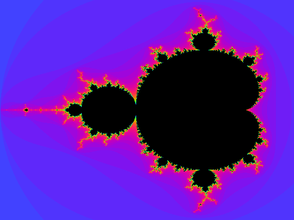
Zooming in
The Mandelbrot set has infinite detail at every scale. Here’s a zoom into the “Seahorse Valley”:
(def mandelbrot-zoom
  (let [h 450 w 600 max-iter 100
        counts (mandelbrot-counts -0.77 -0.73 0.05 0.08 h w max-iter)]
    (counts->image counts h w max-iter)))
(bufimg/tensor->image mandelbrot-zoom)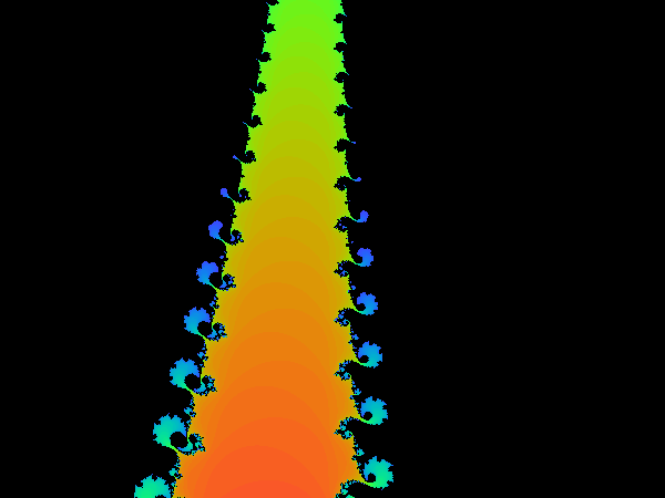
Julia sets
A Julia set uses a fixed \(c\) and varies the starting point \(z_0\). Each choice of \(c\) produces a different fractal.
(def julia-counts
  (fn [c-re c-im re-min re-max im-min im-max h w max-iter]
    (let [z0 (complex-grid re-min re-max im-min im-max h w)
          c-grid (t/complex-tensor
                  (t/compute-tensor [h w 2]
                                    (fn [_ _ part] (if (zero? part) c-re c-im))
                                    :float64))]
      (loop [z z0 counts (t/zeros h w) k 0]
        (if (>= k max-iter)
          counts
          (let [z2 (t/materialize (el/+ (el/* z z) c-grid))
                mask (el/<= (el/abs z2) 2.0)]
            (recur z2 (t/materialize (el/+ counts mask)) (inc k))))))))
Gallery of Julia sets
Different values of \(c\) produce different shapes.
\(c = -0.7 + 0.27i\) — a dendrite (connected, empty interior):
(def julia-dendrite
  (let [h 600 w 600 max-iter 80
        counts (julia-counts -0.7 0.27 -1.5 1.5 -1.5 1.5 h w max-iter)]
    (counts->image counts h w max-iter)))
(bufimg/tensor->image julia-dendrite)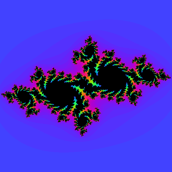
\(c = 0.355 + 0.355i\) — a connected Julia set:
(def julia-connected
  (let [h 600 w 600 max-iter 80
        counts (julia-counts 0.355 0.355 -1.5 1.5 -1.5 1.5 h w max-iter)]
    (counts->image counts h w max-iter)))
(bufimg/tensor->image julia-connected)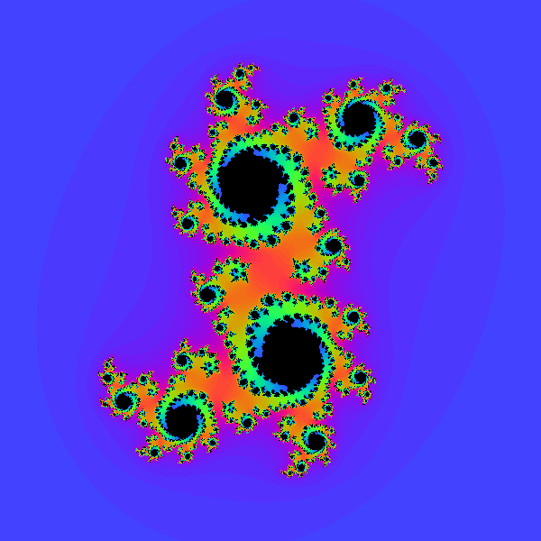
\(c = -0.4 + 0.6i\) — a rabbit-like Julia set:
(def julia-rabbit
  (let [h 600 w 600 max-iter 80
        counts (julia-counts -0.4 0.6 -1.5 1.5 -1.5 1.5 h w max-iter)]
    (counts->image counts h w max-iter)))
(bufimg/tensor->image julia-rabbit)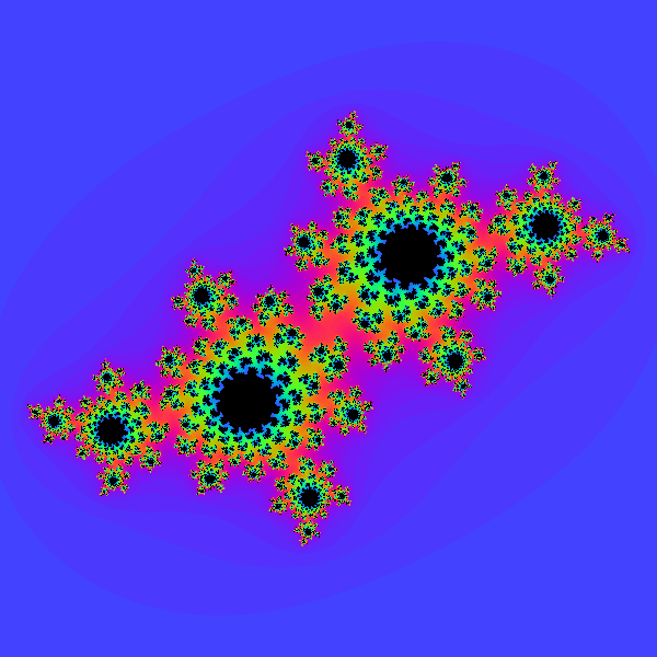
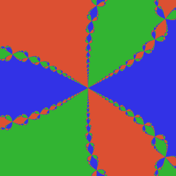
Newton’s fractal
Newton’s method finds roots of equations by iterating \(z_{n+1} = z_n - f(z_n) / f'(z_n)\). In the complex plane, each starting point converges to one of the roots — and the boundaries between convergence regions form a fractal.
We apply Newton’s method to \(f(z) = z^3 - 1\), whose roots are the three cube roots of unity: \(\omega_0 = 1\), \(\omega_1 = e^{2\pi i/3}\), \(\omega_2 = e^{4\pi i/3}\). Since \(f'(z) = 3z^2\), the iteration is:
\[z_{n+1} = z - \frac{z^3 - 1}{3z^2}\]
The division uses el//, which handles complex inputs natively — no need for a manual formula.
(def newton-roots
  (fn [re-min re-max im-min im-max h w max-iter]
    (let [z0 (complex-grid re-min re-max im-min im-max h w)
          ;; Constant grid of 1 + 0i
          one (t/complex-tensor
               (t/compute-tensor [h w 2]
                                 (fn [_ _ part] (if (zero? part) 1.0 0.0))
                                 :float64))
          ;; The three cube roots of unity
          roots [(t/complex 1.0 0.0)
                 (t/complex (math/cos (/ (* 2.0 math/PI) 3.0))
                            (math/sin (/ (* 2.0 math/PI) 3.0)))
                 (t/complex (math/cos (/ (* 4.0 math/PI) 3.0))
                            (math/sin (/ (* 4.0 math/PI) 3.0)))]]
      ;; Iterate Newton's method: z_{n+1} = z - (z³ - 1) / (3z²)
      (let [z-final (loop [z (t/clone z0) k 0]
                      (if (>= k max-iter)
                        z
                        (let [z2 (el/* z z)
                              z3 (el/* z z2)
                              fz (el/- z3 one)
                              fpz (el/scale z2 3.0)]
                          (recur (t/materialize (el/- z (el// fz fpz)))
                                 (inc k)))))
            ;; Classify: compute distance to each root as a tensor
            dists (mapv (fn [root]
                          (let [root-grid (t/complex-tensor
                                           (t/compute-tensor
                                            [h w 2]
                                            (fn [_ _ part]
                                              (if (zero? part)
                                                (double (el/re root))
                                                (double (el/im root))))
                                            :float64))]
                            (el/abs (el/- z-final root-grid))))
                        roots)]
        ;; Pick nearest root per pixel
        (t/compute-matrix h w
                          (fn [r c]
                            (let [d0 ((dists 0) r c)
                                  d1 ((dists 1) r c)
                                  d2 ((dists 2) r c)]
                              (cond
                                (and (<= d0 d1) (<= d0 d2)) 0.0
                                (and (<= d1 d0) (<= d1 d2)) 1.0
                                :else 2.0))))))))
Rendering
Each pixel is colored by which root it converged to.
(def root-colors
  [[230 50 50]    ;; root 0 (1+0i) — red
   [50 180 50]    ;; root 1 — green
[50 80 220]]) ;; root 2 — blue(def roots->image
(fn [root-idx h w]
(t/compute-tensor [h w 3]
(fn [r c ch]
(let [idx (long (root-idx r c))]
(if (neg? idx) 0
(nth (nth root-colors idx) ch))))
:uint8)))The full view
(def newton-img
  (let [h 600 w 600 max-iter 30
        root-idx (newton-roots -2.0 2.0 -2.0 2.0 h w max-iter)]
    (roots->image root-idx h w)))
(bufimg/tensor->image newton-img)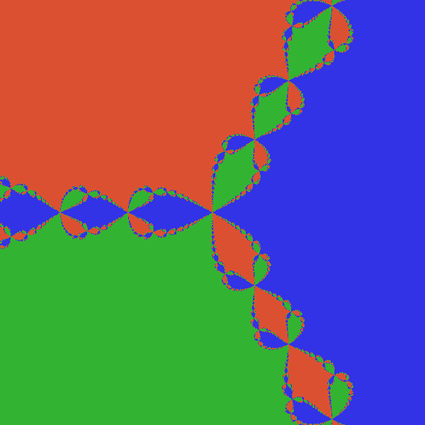
Zooming in
The boundary between basins has fractal detail at every scale.
(def newton-zoom
  (let [h 600 w 600 max-iter 50
        root-idx (newton-roots -0.5 0.5 -0.5 0.5 h w max-iter)]
    (roots->image root-idx h w)))
(bufimg/tensor->image newton-zoom)